Next step is to add in triangles. From there we can go to meshes of triangles, and then render something a bit more interesting than a sphere...

Triangles

As with previous shapes to render a triangle we need to be able to calculate if a ray intersects it or not. There are lots of ray-triangle intersection algorithms out there; the one I have chosen to use is the Möller–Trumbore intersection algorithm as it's fairly quick and also gives us the intersection point in barycentric coordinates which will come in useful later on. I won't go into details of the algorithm here; Scratchapixel has a good discussion of it.

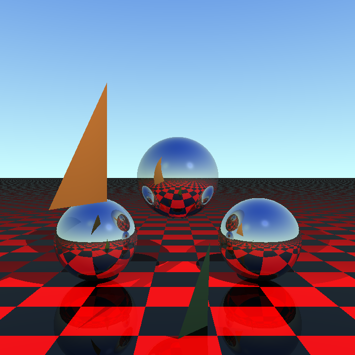
The one other thing we need to calculate is the surface normal. This is easy to do - we have the three points defining our triangle's vertices. From there we can calculate two vectors describing two of the sides. (This is needed for the intersection algorithm anyways) The cross product of two vectors gives a vector perpendicular to both - this will give us the normal we need. With this we can then add some triangles to our scene:

Meshes

A mesh is basically just a collection of triangles, and that's how I've implemented it. I haven't yet attempted to optimise the storage, so there is a lot of repetition because each triangle shares some points with other triangles and these are duplicated rather than stored just once. Intersections with a mesh are straightforward - I can just loop over all the triangles inside the mesh and find the nearest intersection from them, if there is one. This can be slow however as some meshes will contain lots of triangles.

One easy optimisation is to pre-calculate a bounding box for all of the triangles. Luckily we already have an [axis-aligned box](7 - Transparent Boxes#Axis Aligned Box) that we can use for this purpose. Finding the bounding box for a set of points is straightforward because our box is defined in terms of a minimum and maximum point. We therefore loop through all the points in our mesh, find the minimum and maximum values for each axis and then use them to create the box. Our intersection test can then test the box first, and only if it intersects do we then loop through the triangles.

So we have a mesh class - where do we get the mesh data from?

Wavefront .obj Files

Wavefront .obj files are a common and simple way to describe 3D models. Whilst they can contain all manner of geometry I'm only going to worry about simple vertices and faces for now. The files are text and contain lists of vertices followed by faces, e.g.:

v 0.000000 0.000000 0.000000
v 0.000000 0.000000 1.000000
v 0.000000 1.000000 1.000000
f 1 2 3

The v lines give the vertex coordinates, in this case \( \big(0, 0, 0 \big) \), \( \big(0, 0, 1 \big) \) and \( \big(0, 1, 1 \big) \). The f lines represent faces made up of three or more vertices - the numbers references the previously defined vertices, so in this case the f line represents a triangle made up from the three vertices.

The f lines can represent polygons of any number of sides, however it's easy to break them up into triangles by creating a fan of triangles around the first vertex in the face.

The only problem with the above is that the vertices could describe an object of any size in any position in 3D space. We need some way to move the object to a position of our choosing. An easy way to do that is with transformation matrices.

Transformation Matrices

We can represent various transformations such as rotations, scaling and translations with a 4x4 [matrix](https://en.wikipedia.org/wiki/Matrix_(mathematics). By taking a matrix that represents our transformation and multiplying it with a 4D vector that represents our 3D vector or point in homogeneous coordinates we get a new 4D vector representing the transformed vector/point. Turning our vectors and points to 4D homogeneous coordinates is simple - we simply add an extra component that is 1 for point or 0 for a vector:

• Point \( \big( 3, 4, 2 \big) \) becomes \( \big(3, 4, 2, 1 \big) \)
• Vector \( \hat{\mathbf{i}} + 2 \hat{\mathbf{j}} - 3 \hat{\mathbf{k}}\) becomes \( \big(1, 2, -3, 0 \big) \)

The 0 for vectors effectively ignores any translation in our transformation matrix - as a vector represents a direction only it makes no sense to translate it. Points represent a position so translating them does have a meaning, and the 1 keeps the translation components in place. To convert back after the transform we just drop the last component.

Combining transformations together into a single matrix is also straightforward - we simply multiply them together. The order of matrix multiplication is important and the second transformation comes first in the multiplication. For example to apply a rotation \( \mathsf{R} \) followed by a translation \( \mathsf{T} \) we would use the matrix \( \mathsf{TR} \).

I've added a Matrix class to represent a 4x4 matrix. As well as operators to represent standard matrix operations such as add and multiply it has methods to transform points and vector as well as static methods to generate matrices representing common transformations:

Translation

Translation is the identity matrix with the translation in \( x \), \( y \) and \( z \) axes along the bottom row of the matrix:

\[ \begin{bmatrix} 1 & 0 & 0 & 0 \\ 0 & 1 & 0 & 0 \\ 0 & 0 & 1 & 0 \\ x & y & z & 1 \end{bmatrix} \]

Scaling

For scaling we place the factor to scale by (1 being remain the same, larger increase size, smaller reduce size) for each axis along the diagonal with a 1 in the bottom right:

\[ \begin{bmatrix} x & 0 & 0 & 0 \\ 0 & y & 0 & 0 \\ 0 & 0 & z & 0 \\ 0 & 0 & 0 & 1 \end{bmatrix} \]

Rotation

We can define a matrix for rotating about each axis, with respect to the origin. If our angles are in radians then we have the following three matrices for rotating \( \theta \) radians about \( x \), \( y \) and \( z \) respectively:

\[ \begin{bmatrix} 1 & 0 & 0 & 0 \\ 0 & \cos\theta & \sin\theta & 0 \\ 0 & -\sin\theta & \cos\theta & 0 \\ 0 & 0 & 0 & 1 \end{bmatrix} \]

\[ \begin{bmatrix} \cos\theta & 0 & -\sin\theta & 0 \\ 0 & 1 & 0 & 0 \\ \sin\theta & 0 & \cos\theta & 0 \\ 0 & 0 & 0 & 1 \end{bmatrix} \]

\[ \begin{bmatrix} \cos\theta & \sin\theta & 0 & 0 \\ -\sin\theta & \cos\theta & 0 & 0 \\ 0 & 0 & 1 & 0 \\ 0 & 0 & 0 & 1 \end{bmatrix} \]

Normalising a Mesh

I've added a method to our Mesh class that can 'normalise' it. By normalise I mean:

• Translate it so that the minimum point of the mesh's axis-aligned bounding box is (0, 0, 0). We have an axis-aligned bounding box for the raw mesh; we simply translate by the negative of the minimum point for that. So if they minimum was \( \big( -5, 4, 2 \big) \) we would translate by 5, -4 and 2 for \( x \), \( y \) and \( z \) axes respectively.
• Scale it so it fits inside an axis-aligned bounding box of width, depth and height 1. From the axis-aligned box for the raw mesh we find the longest side and then scale by the inverse of that. So if our box had width = 3, height = 4 and depth = 5 we would take the longest side (5) and scale by the inverse of that, i.e. 1/5.

Once it is normalised it's much easier to perform further translations to position the mesh in the scene. We are now in a position to do an obligatory render of the classic Utah Teapot; here I've rendered a mesh of the teapot from http://goanna.cs.rmit.edu.au/~pknowles/models.html:

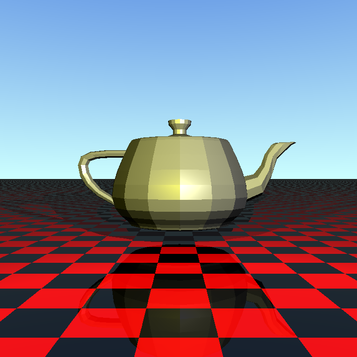
Rendering a Smooth Mesh

Given the teapot is a mesh of triangles it's not surprising that it looks like a mesh of triangles. It would be nicer if we had a smooth teapot. One way to do that is to define normals at each of the vertices and then interpolate them over the triangle. .obj files support vertex normals via lines beginning vn. Our previous example with vertex normals might look like this:

v 0.000000 0.000000 0.000000
v 0.000000 0.000000 1.000000
v 0.000000 1.000000 1.000000
vn 1.000000 1.000000 0.000000
vn 0.000000 1.000000 1.000000
vn 1.000000 .000000 1.000000
f 1//1 2//2 3//3

The face now points to both the vertex and the normal at the vertex. (The missing number between the backslashes would be the texture coordinate for the vertex; this will come in useful when I implement texture mapping) One thing to note is that the normals aren't necessarily normalized in .obj files so we need to do that ourselves.

How do we interpolate these normals though? As well as giving the point on the ray of the intersection the Möller–Trumbore algorithm also gives us the point on the surface in terms of the barycentric coordinates \( u \) and \( v \). A point \( P \) on the triangle with corners \( A \), \( B \) and \( C \) can be described as:

\[ P = wA + uB + vC \]

However \( u + v + w = 1 \), so we have:

\[ P = (1 - u - v)A + uB + vC \]

I.e. the three barycentric coordinates for a point describe how close to each of the three corners the point is. We can use this when interpolating our vertex normals; if the point is closer to one of the vertices then it's normal will have a greater contribution in the interpolation. We can just swap our vertex normals into the above equation:

\[ \mathbf{N} = (1 - u - v)\mathbf{N_A} + u\mathbf{N_B} + v\mathbf{N_C} \]

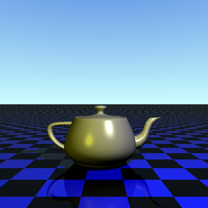
Plugging all this into our renderer gives us a nice smooth teapot:

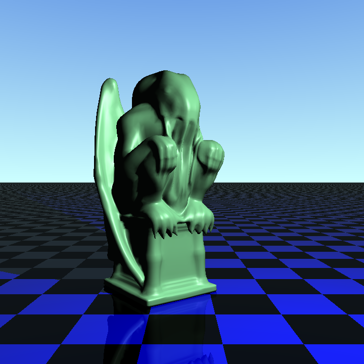
We render more complex objects too, such as this excellent Cthulhu Statuette by Samize:

The code so far can be found on GitHub.